11. Scipy Tutorial-多维插值griddata
scipy.interpolate模块下的griddata函数可以处理多元(维)函数的插值,以二元函数$f(x, y)$为例说明一下griddata的使用。与之前的一元函数插值interp1d相区别,interp1d是通过已知的点集$P = {(x_i, y_i)|x_i \in R, y_i \in R }$通过interp1d可以找到一个函数$f(x_i) = y_i$,那么任何一个$x_j$通过插值函数就能求得其$y_j = f(x_j)$,$y_i$即插值,这里的$x_j$可能是点集P里的一个数据,也可以不是,这是一元插值的思想。可以看出插值需要$f(x)$算出来,而griddata函数可以用于多元的插值,其返回值不是一个函数,而是插值本身,可以通过下面的代码验证一下这个说法。
下面的代码看上去很长,实际内容并不多,大致有三部分:第一部分从import numpy as np语句开始,到import matplotlib.pyplot as plt,这部分是本例子的核心,即求多元数据的插值,使用了griddata函数。第二部分是数据的可视化,从语句import matplotlib.pyplot as plt开始到第一个plt.show()即第一次数据可视化输出,这部分的作用是绘制已知点集和插值的数据的可视化。第三部分 从print "*" * 20语句开始一直到程序结束,这部分主要是验证griddata函数返回的是插值数据本身,无需像一元interp1d插值那样用点去计算插值了,返回值本身就是插值数据。
import numpy as np
def func(x, y):
    return x*(1-x)*np.cos(4*np.pi*x) * np.sin(4*np.pi*y**2)**2
grid_x, grid_y = np.mgrid[0:1:100j, 0:1:200j]
points = np.random.rand(1000, 2)
values = func(points[:,0], points[:,1])

from scipy.interpolate import griddata
grid_z0 = griddata(points, values, (grid_x, grid_y), method='nearest')
grid_z1 = griddata(points, values, (grid_x, grid_y), method='linear')
grid_z2 = griddata(points, values, (grid_x, grid_y), method='cubic')

import matplotlib.pyplot as plt
from mpl_toolkits.mplot3d.axes3d import Axes3D
plt.figure()

ax1 = plt.subplot2grid((2,2), (0,0), projection='3d')
ax1.plot_surface(grid_x, grid_y, grid_z0, color = "c")
ax1.set_xlim3d(0, 1)
ax1.set_ylim3d(0, 1)
ax1.set_zlim3d(-0.25, 0.25)
ax1.set_title('nearest')

ax2 = plt.subplot2grid((2,2), (0,1), projection='3d')
ax2.plot_surface(grid_x, grid_y, grid_z1, color = "c")
ax2.set_xlim3d(0, 1)
ax2.set_ylim3d(0, 1)
ax2.set_zlim3d(-0.25, 0.25)
ax2.set_title('linear')

ax3 = plt.subplot2grid((2,2), (1,0), projection='3d')
ax3.plot_surface(grid_x, grid_y, grid_z2, color = "r")
ax3.set_xlim3d(0, 1)
ax3.set_ylim3d(0, 1)
ax3.set_zlim3d(-0.25, 0.25)
ax3.set_title('cubic')

ax4 = plt.subplot2grid((2,2), (1,1), projection='3d')
ax4.scatter(points[:,0], points[:,1], values,  c= "b")
ax4.set_xlim3d(0, 1)
ax4.set_ylim3d(0, 1)
ax4.set_zlim3d(-0.25, 0.25)
ax4.set_title('org_points')

plt.tight_layout()
plt.show()

print "*" * 20

ax1 = plt.subplot2grid((2,2), (0,0), projection='3d')
ax1.plot_surface(grid_x, grid_y, grid_z1, color = "c")
ax1.scatter(points[:,0][:100], points[:,1][:100], values[:100],  c= "r", s = 20)
ax1.set_xlim3d(0, 1)
ax1.set_ylim3d(0, 1)
ax1.set_zlim3d(-0.25, 0.25)
ax1.set_title('org_points')

x = np.linspace(0, 1.00, num = 10, endpoint=True)
y = np.linspace(0, 0.5, num = 10, endpoint=True)
x,y = np.meshgrid(x, y)
ax2 = plt.subplot2grid((2,2), (0,1), projection='3d')
ax2.plot_surface(grid_x, grid_y, grid_z1, color = "c")
ax2.scatter(x, y, func(x, y),  c= "b", s = 20)
y = np.linspace(0.5, 1.0, num = 10, endpoint=True)
x,y2 = np.meshgrid(x, y)
ax2.scatter(x, y2, func(x, y2),  c= "b", s = 20)
ax2.set_xlim3d(0, 1)
ax2.set_ylim3d(0, 1)
ax2.set_zlim3d(-0.25, 0.25)
ax2.set_title('meshgrid')


x = np.linspace(0, 1.00, num = 10, endpoint=True)
y = np.linspace(0, 0.5, num = 10, endpoint=True)
x,y = np.meshgrid(x, y)
ax3 = plt.subplot2grid((2,2), (1,0), projection='3d')
ax3.scatter(points[:,0][:100], points[:,1][:100], values[:100],  c= "r", s = 20)
ax3.scatter(x, y, func(x, y),  c= "b", s = 20)
y = np.linspace(0.5, 1.0, num = 10, endpoint=True)
x,y2 = np.meshgrid(x, y)
ax3.scatter(x, y2, func(x, y2),  c= "b", s = 20)
#ax3.plot_wireframe
ax3.plot_surface(grid_x, grid_y, grid_z1, color = "c",alpha=0.5)
ax3.set_xlim3d(0, 1)
ax3.set_ylim3d(0, 1)
ax3.set_zlim3d(-0.25, 0.25)
ax3.set_title('org_point and meshgrid')

plt.tight_layout()
plt.show()
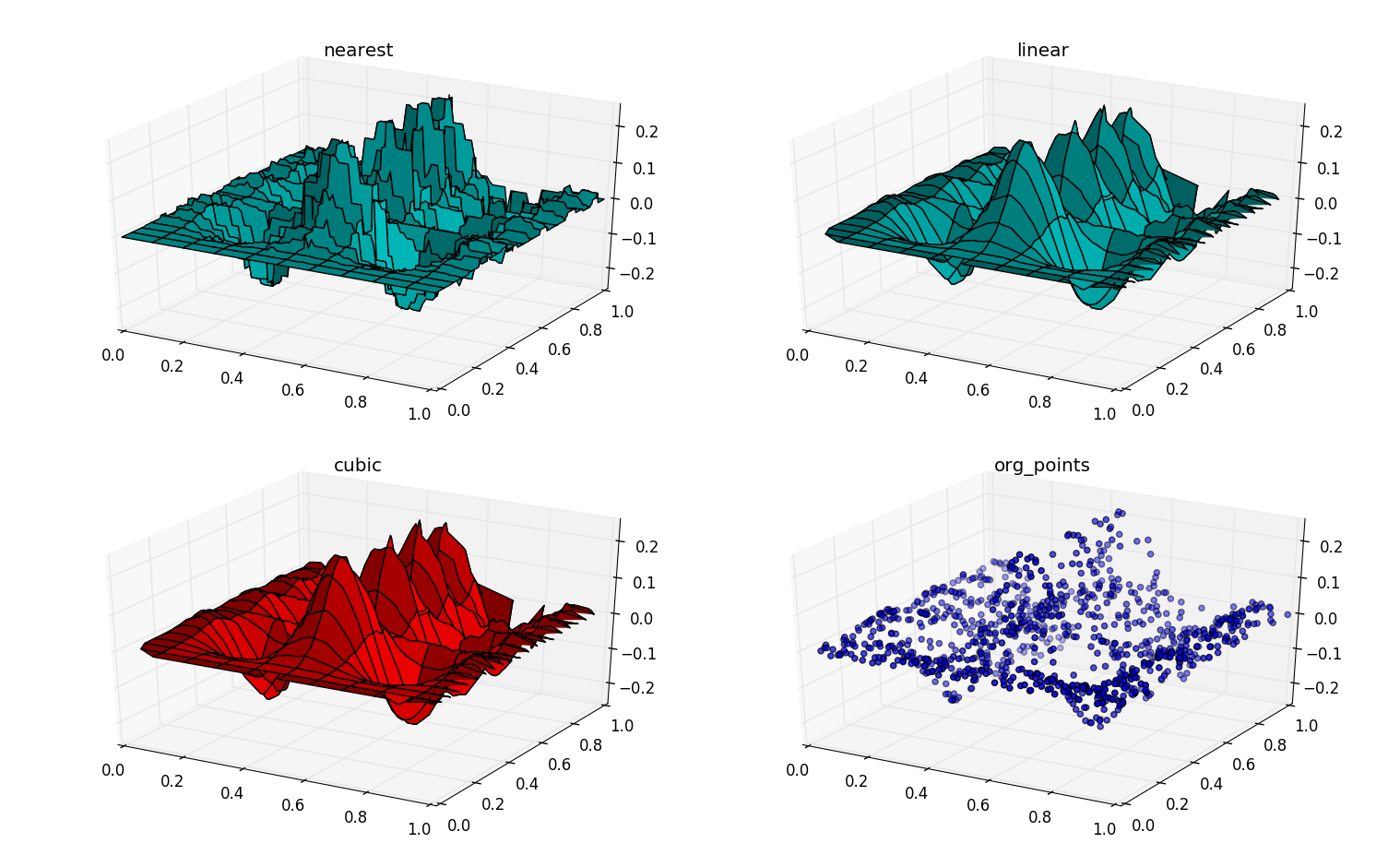
程序输出的第一副图,展示是用不同的插值方法对多元数据进行插值的效果如何,图内左上图是method=nearest的插值效果,右上图为method=linear的插值效果,左下图是method=cubic的插值效果,右下图则是已知的多元点集散点图。
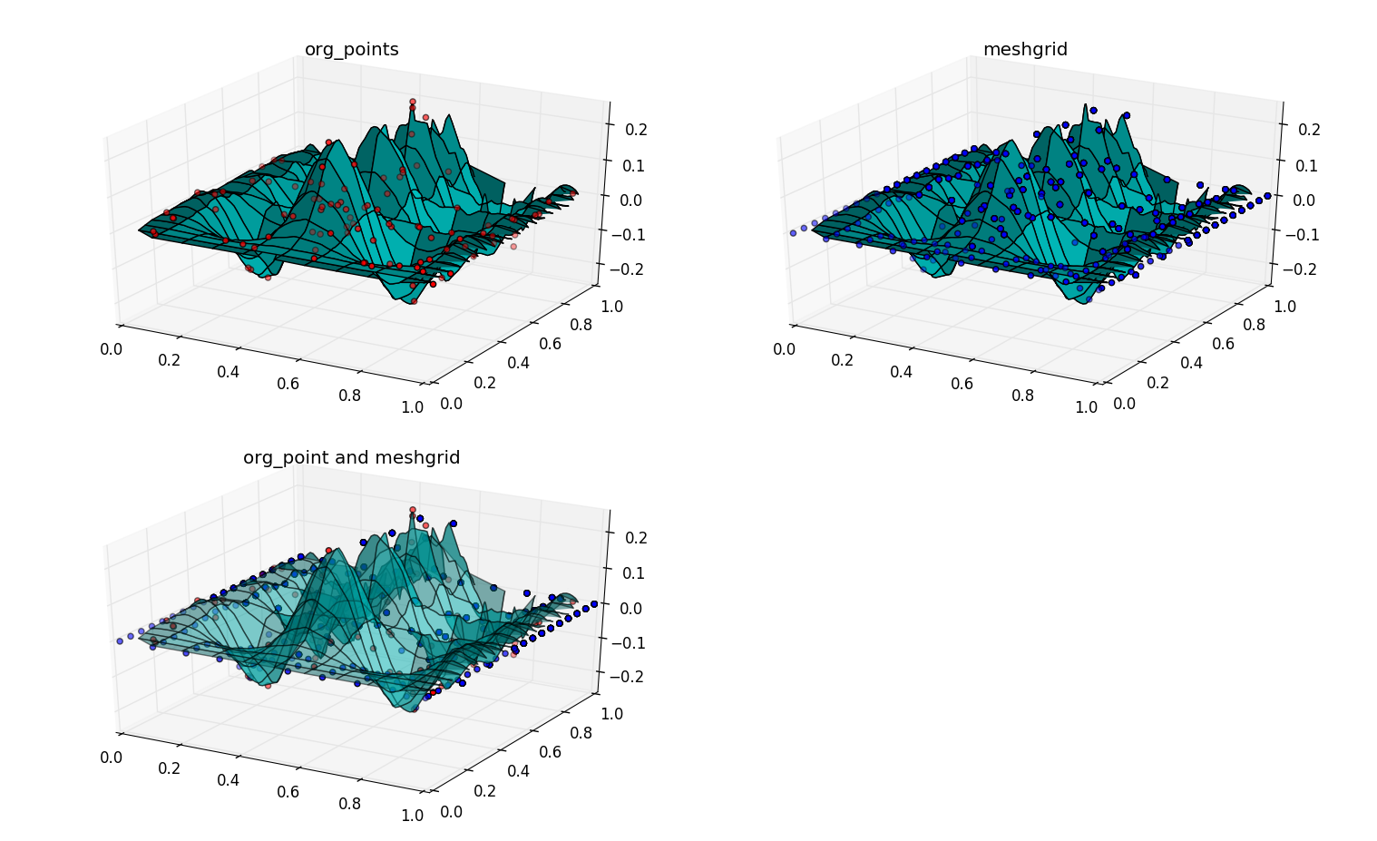
 程序的第二个输出图是下图,左上图反应的是插值结果(曲面的形式)和已知点集(散点的形式)里100个数据可视化。右上图是插值结果(曲面)和$f(x_i,y_i)$计算结果(散点)的可视化图。右下图则是插值结果(曲面)和已知点集(散点,红色)以及$f(x_i,y_i)$计算结果(散点,蓝色)的可视化图。
 下面分三小节来说明一下程序。
- 程序的第一部分是用griddata求多元插值。
import numpy as np
def func(x, y):
    return x*(1-x)*np.cos(4*np.pi*x) * np.sin(4*np.pi*y**2)**2
grid_x, grid_y = np.mgrid[0:1:100j, 0:1:200j]
points = np.random.rand(1000, 2)
values = func(points[:,0], points[:,1])

from scipy.interpolate import griddata
grid_z0 = griddata(points, values, (grid_x, grid_y), method='nearest')
grid_z1 = griddata(points, values, (grid_x, grid_y), method='linear')
grid_z2 = griddata(points, values, (grid_x, grid_y), method='cubic')
前边已经说了griddata的结果是插值不是函数,那是谁的插值呢?
grid_z0 = griddata(points, values, (grid_x, grid_y), method='nearest')
调用函数griddata时一共传入了四个参数:
(1).points代表已知多元的点集,这里展示的是二元的所以是$(x_i, y_i)$共1000个,是通过points = np.random.rand(1000, 2)语句实现的,其形状是$[1000, 2]$或$1000 \times 2$的矩阵,即1000个平面上的点。
(2).第二个参数是values,是通过调用func函数计算的结果。func函数实现的是如下公式的计算: $$ z = f(x,y) = x(1-x)\cos(4\pi x)\sin(4\pi y^2)^2 $$
(3). 第三个参数是一个元组(grid_x, grid_y),是由语句grid_x, grid_y = np.mgrid[0:1:100j, 0:1:200j]产生的,mgrid函数之前已经介绍过,可以产生坐标点集。
import matplotlib.pyplot as plt
import numpy as np
x, y = np.mgrid[1:3:3j, 10:12:3j]
print "*" * 10
print x
print "*" * 10
print y
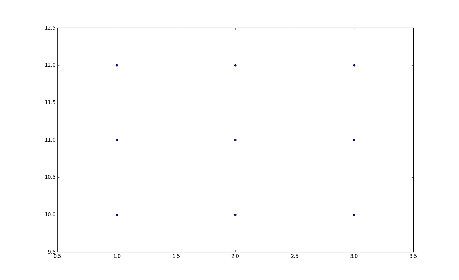
plt.scatter(x, y)
plt.show()
图像输出结果:
 程序执行打印结果:
**********
[[1. 1. 1.]
 [2. 2. 2.]
 [3. 3. 3.]]
**********
[[10. 11. 12.]
 [10. 11. 12.]
 [10. 11. 12.]]
当$x_0 = 1$时$y_0 = 10,y_1 = 11,y_2 = 12$即上图最左边的三个点。
(4).第四个参数是method的设置,即插值的方法,grid_z0用的是'nearest',grid_z1用的是'linear'一次线性,,grid_z0用的是'cubic'三次插值。
第三个参数是元组(grid_x, grid_y)放在这儿有何意义?前两个参数相当与interp1d里的$x_i$和$y_i$的作用,有这两个参数就能够预测找到一个合适的函数来包含已知点集了,那第三个参数给出来不就多余了么?实际上确实如此,但估计找到的函数过于复杂,调用起来不方便,既然是研究插值,那么直接在找函数的同时直接给出插值岂不更好?所以griddata的第三个参数有点像一元插值思想里提及的$f(x_j)$的意图,即griddata不是找函数,而是直接求得插值。
- 程序的第二部分是插值可视化。
import matplotlib.pyplot as plt
from mpl_toolkits.mplot3d.axes3d import Axes3D
plt.figure()

ax1 = plt.subplot2grid((2,2), (0,0), projection='3d')
#print "ax1", type(ax1)
ax1.plot_surface(grid_x, grid_y, grid_z0, color = "c")
ax1.set_xlim3d(0, 1)
ax1.set_ylim3d(0, 1)
ax1.set_zlim3d(-0.25, 0.25)
ax1.set_title('nearest')

ax2 = plt.subplot2grid((2,2), (0,1), projection='3d')
ax2.plot_surface(grid_x, grid_y, grid_z1, color = "c")
ax2.set_xlim3d(0, 1)
ax2.set_ylim3d(0, 1)
ax2.set_zlim3d(-0.25, 0.25)
ax2.set_title('linear')

ax3 = plt.subplot2grid((2,2), (1,0), projection='3d')
ax3.plot_surface(grid_x, grid_y, grid_z2, color = "r")
ax3.set_xlim3d(0, 1)
ax3.set_ylim3d(0, 1)
ax3.set_zlim3d(-0.25, 0.25)
ax3.set_title('cubic')

ax4 = plt.subplot2grid((2,2), (1,1), projection='3d')
ax4.scatter(points[:,0], points[:,1], values,  c= "b")
ax4.set_xlim3d(0, 1)
ax4.set_ylim3d(0, 1)
ax4.set_zlim3d(-0.25, 0.25)
ax4.set_title('org_points')

plt.tight_layout()
plt.show()
这部分不难,就是用matplot来绘制可视图,subplot2grid函数里通过指定projection='3d'来创建一个Axes3D的实例对象,实现3D可视化。scatter函数要求都是一维的数组(已知的散点points和values)。而plt_surface函数则要求网格坐标即二维数组(grid_x和grid_y、grid_z0等)。
- 第三部分是验证一下griddata的返回值是插值而不是函数,是谁的插值?是(grid_x, grid_y)代表的这个区域的每个点的插值。
print "*" * 20

ax1 = plt.subplot2grid((2,2), (0,0), projection='3d')
ax1.plot_surface(grid_x, grid_y, grid_z1, color = "c")
ax1.scatter(points[:,0][:100], points[:,1][:100], values[:100],  c= "r", s = 20)
ax1.set_xlim3d(0, 1)
ax1.set_ylim3d(0, 1)
ax1.set_zlim3d(-0.25, 0.25)
ax1.set_title('org_points')

x = np.linspace(0, 1.00, num = 10, endpoint=True)
y = np.linspace(0, 0.5, num = 10, endpoint=True)
x,y = np.meshgrid(x, y)
ax2 = plt.subplot2grid((2,2), (0,1), projection='3d')
ax2.plot_surface(grid_x, grid_y, grid_z1, color = "c")
ax2.scatter(x, y, func(x, y),  c= "b", s = 20)
y = np.linspace(0.5, 1.0, num = 10, endpoint=True)
x,y2 = np.meshgrid(x, y)
ax2.scatter(x, y2, func(x, y2),  c= "b", s = 20)
ax2.set_xlim3d(0, 1)
ax2.set_ylim3d(0, 1)
ax2.set_zlim3d(-0.25, 0.25)
ax2.set_title('meshgrid')


x = np.linspace(0, 1.00, num = 10, endpoint=True)
y = np.linspace(0, 0.5, num = 10, endpoint=True)
x,y = np.meshgrid(x, y)
ax3 = plt.subplot2grid((2,2), (1,0), projection='3d')
ax3.scatter(points[:,0][:100], points[:,1][:100], values[:100],  c= "r", s = 20)
ax3.scatter(x, y, func(x, y),  c= "b", s = 20)
y = np.linspace(0.5, 1.0, num = 10, endpoint=True)
x,y2 = np.meshgrid(x, y)
ax3.scatter(x, y2, func(x, y2),  c= "b", s = 20)
#ax3.plot_wireframe
ax3.plot_surface(grid_x, grid_y, grid_z1, color = "c",alpha=0.5)
ax3.set_xlim3d(0, 1)
ax3.set_ylim3d(0, 1)
ax3.set_zlim3d(-0.25, 0.25)
ax3.set_title('org_point and meshgrid')

plt.tight_layout()
plt.show()
(1). 图例有三个子图,ax1代表左上的图,语句:
ax1.plot_surface(grid_x, grid_y, grid_z1, color = "c")
绘制的是griddata计算(grid_x, grid_y)这些数据在points和values已知数据下计算出(grid_x, grid_y)所对应的值的集合grid_z1。而下面的语句:
ax1.scatter(points[:,0][:100], points[:,1][:100], values[:100], c= "r", s = 20)
则是绘制已知points、values的点图(红色散点),原来有1000个已知点,太多就选用了100个,类似一元插值的$x_i$和$y_i$。而grid_z0则类似于$f(x_j) = y_j$。
(2). ax2代表的是右上子图,
x = np.linspace(0, 1.00, num = 10, endpoint=True)
y = np.linspace(0, 0.5, num = 10, endpoint=True)
x,y = np.meshgrid(x, y)
ax2 = plt.subplot2grid((2,2), (0,1), projection='3d')
ax2.plot_surface(grid_x, grid_y, grid_z1, color = "c")
ax2.scatter(x, y, func(x, y),  c= "b", s = 20)
y = np.linspace(0.5, 1.0, num = 10, endpoint=True)
x,y2 = np.meshgrid(x, y)
ax2.scatter(x, y2, func(x, y2),  c= "b", s = 20)
绘制的是用区域(grid_x, grid_y)里的各个点的计算值(蓝色散点)和用points和values求得的插值(曲面)grid_z1的可视化图。 由于scatter要求x和y长度相同的一维数组(n,),grid_x, grid_y是(100,200)的,所以将y轴分为两部分y和y2这样x和y,x和y2都是100,所以scatter了两次(蓝色散点)。 绘制计算值的语句是:
ax2.scatter(x, y, func(x, y),  c= "b", s = 20)
...
ax2.scatter(x, y2, func(x, y2),  c= "b", s = 20)
绘制griddata插值语句:
ax2.plot_surface(grid_x, grid_y, grid_z1, color = "c")
(3).ax3绘制的是右下的3d可视图。 用语句
ax3.scatter(points[:,0][:100], points[:,1][:100], values[:100], c= "r", s = 20)
绘制了已知数据点集里的100个points(红色,散点)。 用语句
ax3.scatter(x, y, func(x, y),  c= "b", s = 20)
ax3.scatter(x, y2, func(x, y2),  c= "b", s = 20)
绘制区域(grid_x, grid_y)里的各个点的计算值(蓝色,散点) 用语句
ax3.plot_surface(grid_x, grid_y, grid_z1, color = "c",alpha=0.5)
绘制的是已知点集获得的(grid_x, grid_y)里的各个点的插值的曲面图。